Data Processing
Data processing is a crucial step in analyzing experimental data using LCDA. Data collected from experiments may contain various issues, such as noise, skewness, and outliers, which may affect the accuracy and reliability of the results. Therefore, it is important to process the data before analysis.
This chapter will guide you through the steps of data processing. Whether you are a novice or an experienced user, this chapter provides valuable information and guidance to help you obtain accurate and reliable results using LCDA.
Data Processing Projects
Create a new project
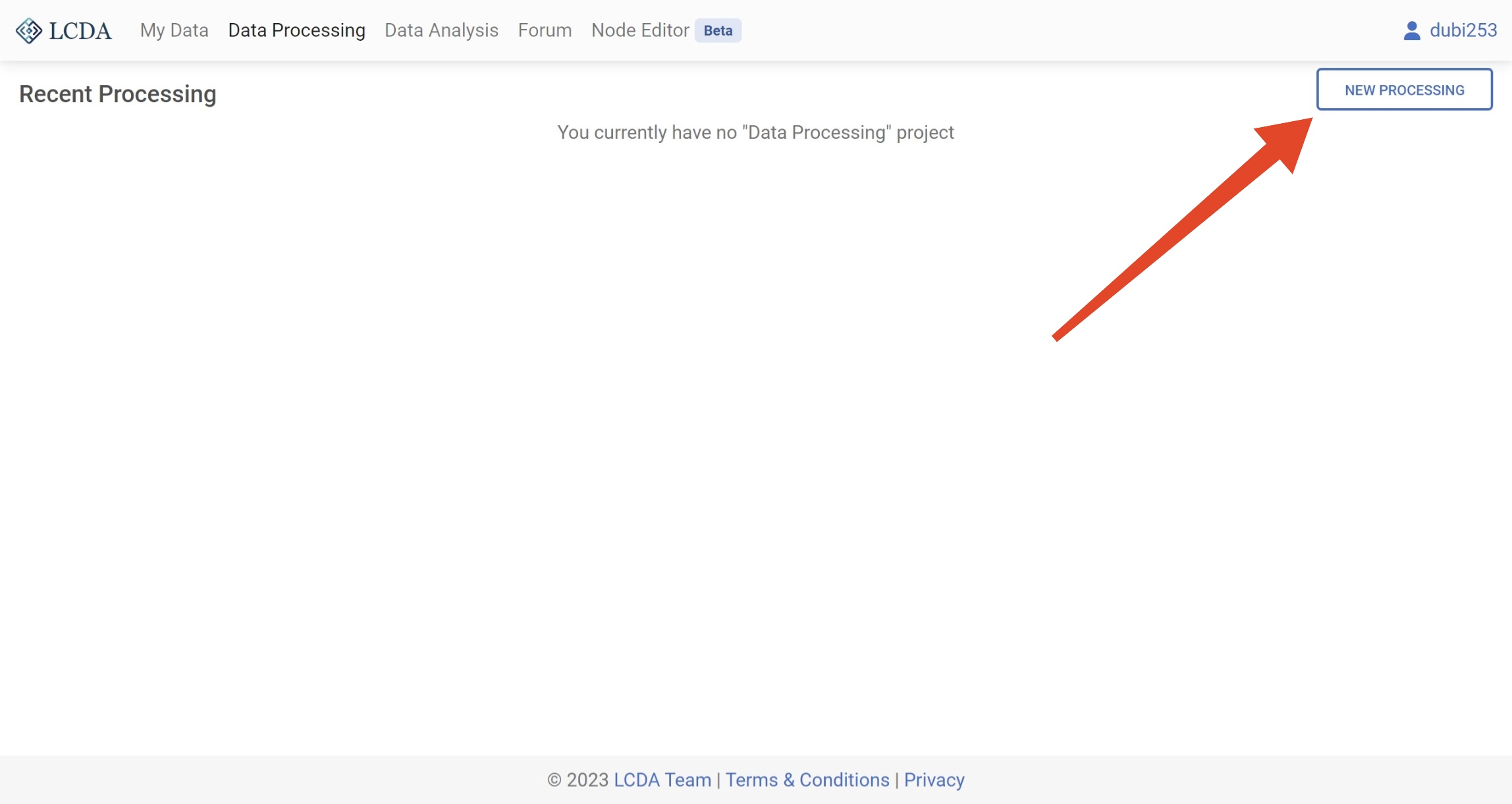
Before beginning data processing in LCDA, you will need to create a new data processing project. This can be done by clicking on the NEW PROCESSING button located in the upper right corner of the Data Processing interface.
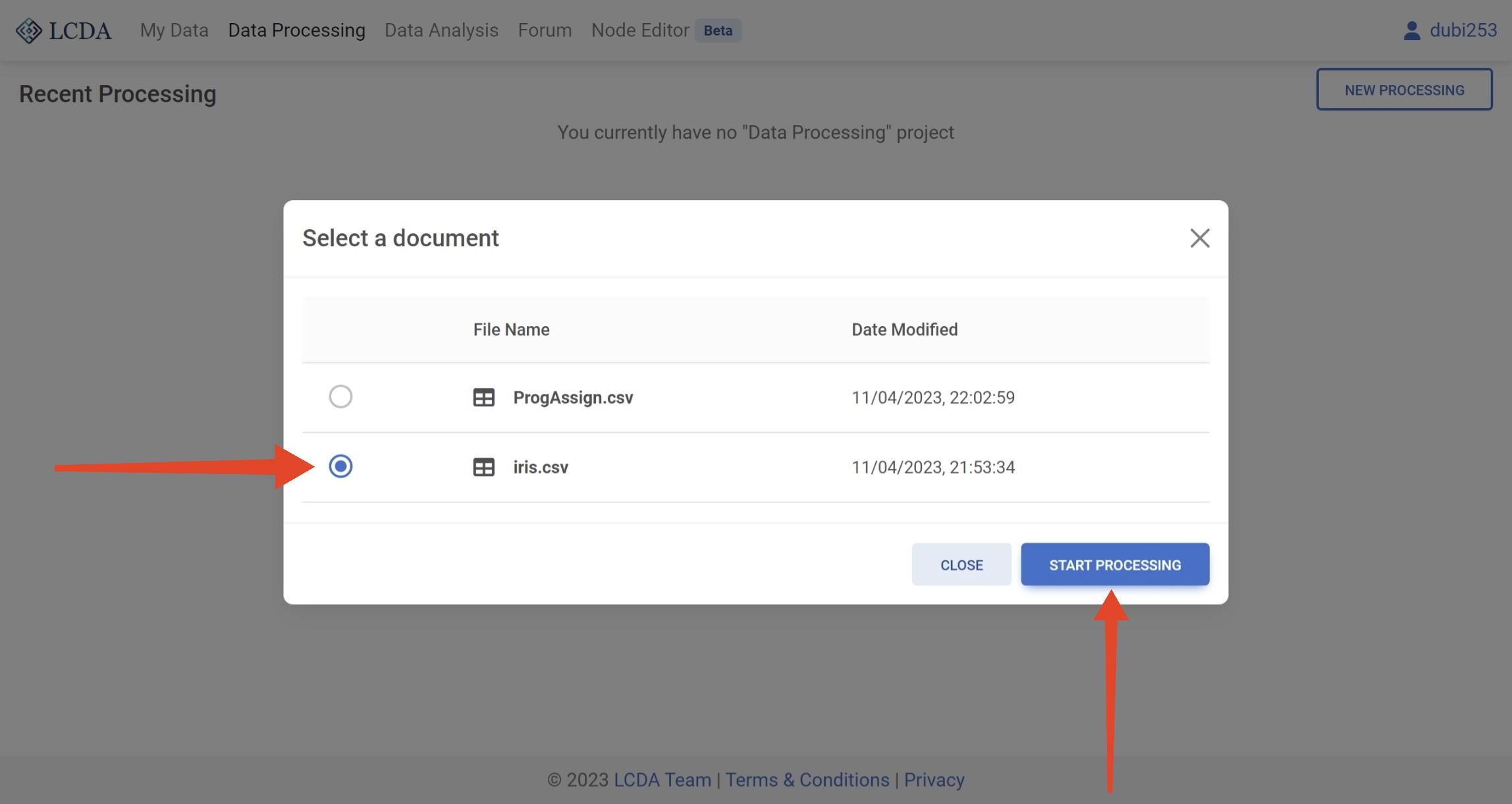
In the pop-up window, you will need to select a dataset (Want to upload your own dataset? Please refer to the My Data user manual to learn how to upload a dataset). Then click on the START PROCESSING button in the lower right corner to start data processing. The system will automatically create a data processing project for you.
Here we use the iris.csv dataset to demonstrate the process of data processing.
Continue editing a project
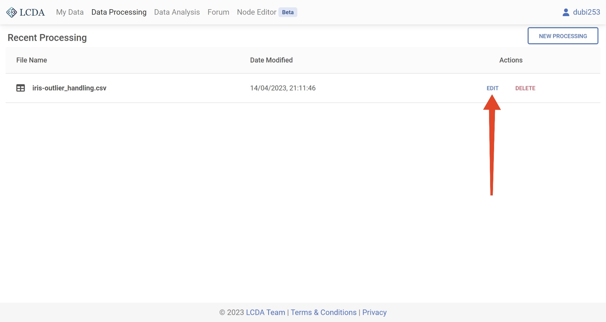
If you have already created a data processing project, the data processing interface will list all of your data processing projects. You can click on the EDIT button on the right to continue editing an existing data processing project.
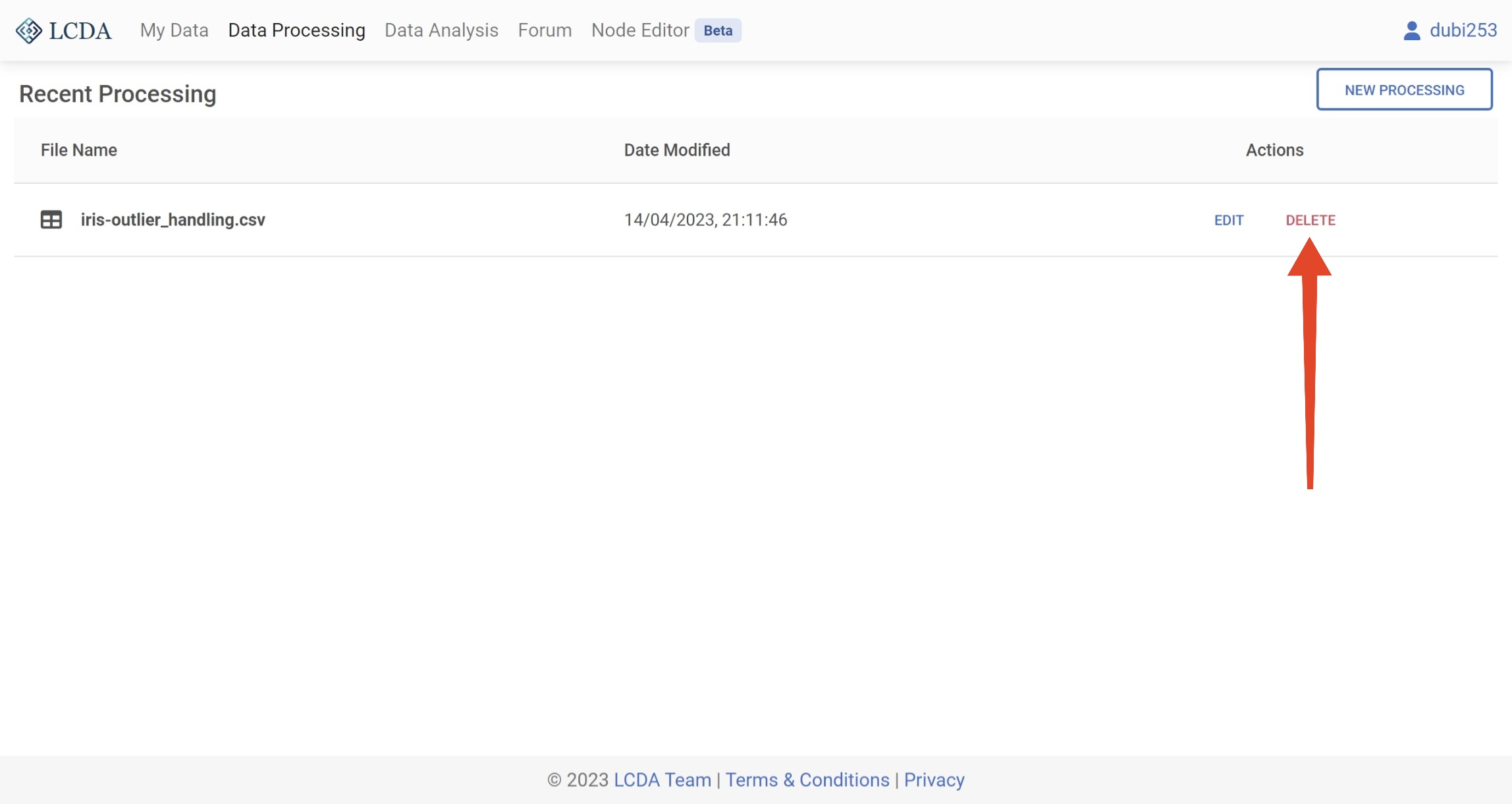
Delete a project
If you no longer need a data processing project, you can click on the DELETE button on the right to delete the project.
WARNING
Note: Deleting data processing items is a permanent operation and cannot be recovered after deletion. This also deletes the dataset generated by the last run in the project. Please make sure you have saved the data you need before deleting the project.
Data Processing Steps
After clicking the
EDITbutton or creating a new data processing project, the data processing interface is displayed. From here, you can work with the data.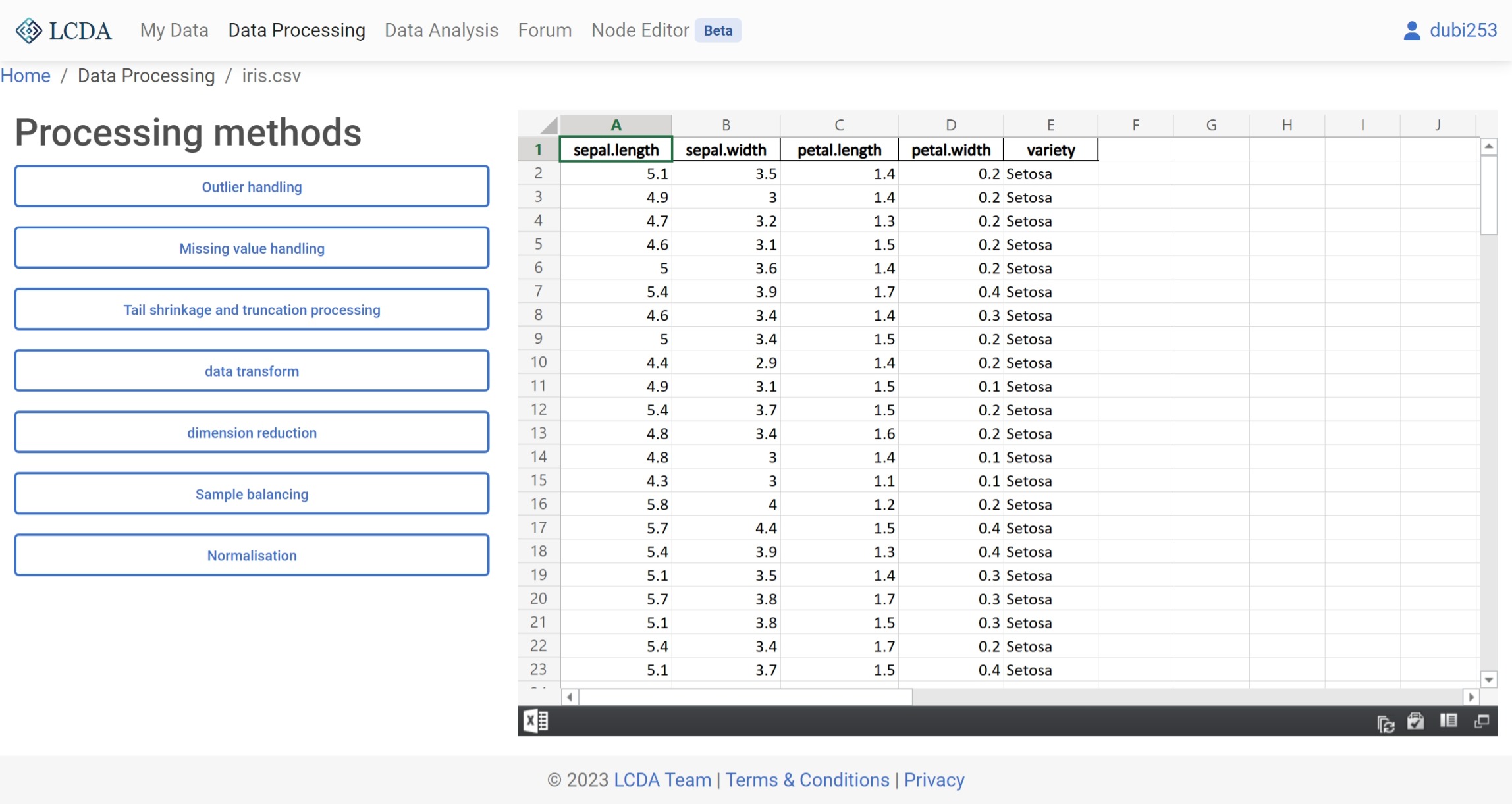
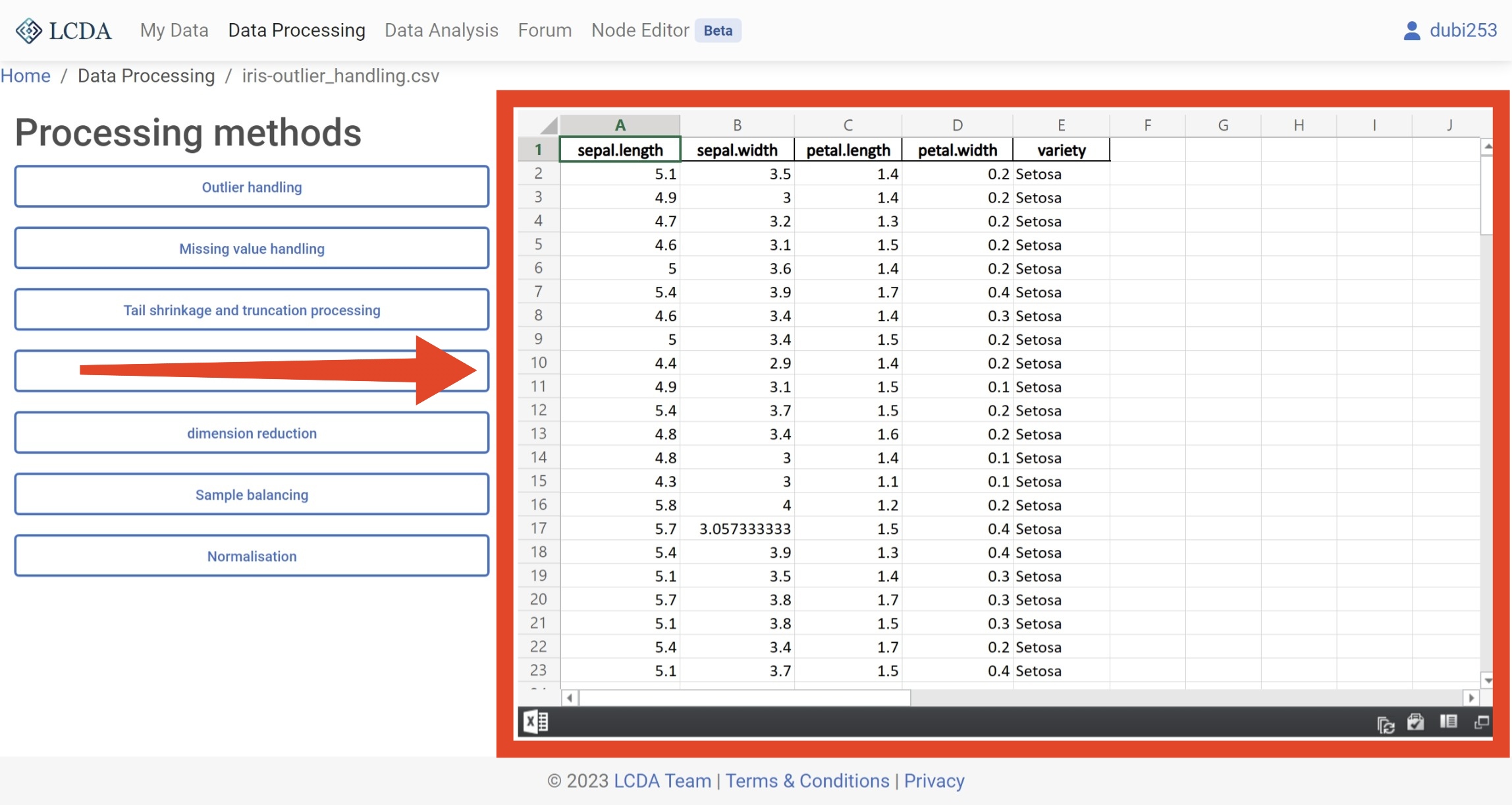
In the data processing interface, you will find a list of data processing algorithms on the left-hand side. You can select the algorithm you want to use by clicking on it, and then set the parameters of the algorithm in the pop-up panel. The specific parameters for each algorithm may vary, so please refer to the Data Processing Algorithms for more information on how to set them.
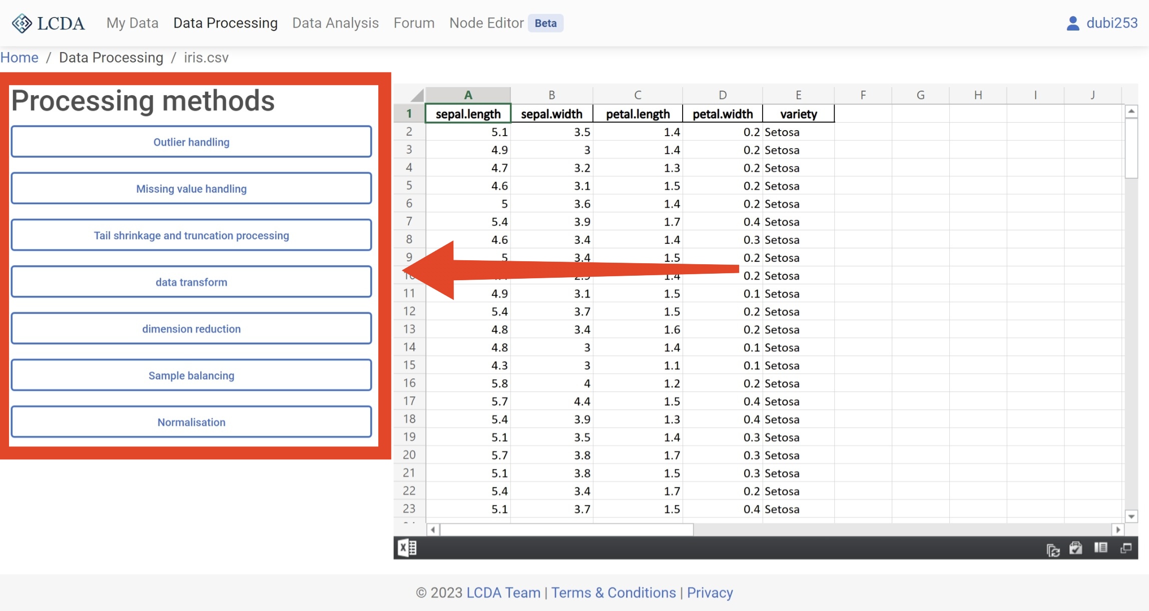
Here, we will demonstrate the process of using the
Outlier handlingalgorithm as an example. Once you have selected the algorithm and set the parameters, you can click on theStart processingbutton located in the lower right corner of the panel to initiate the algorithm.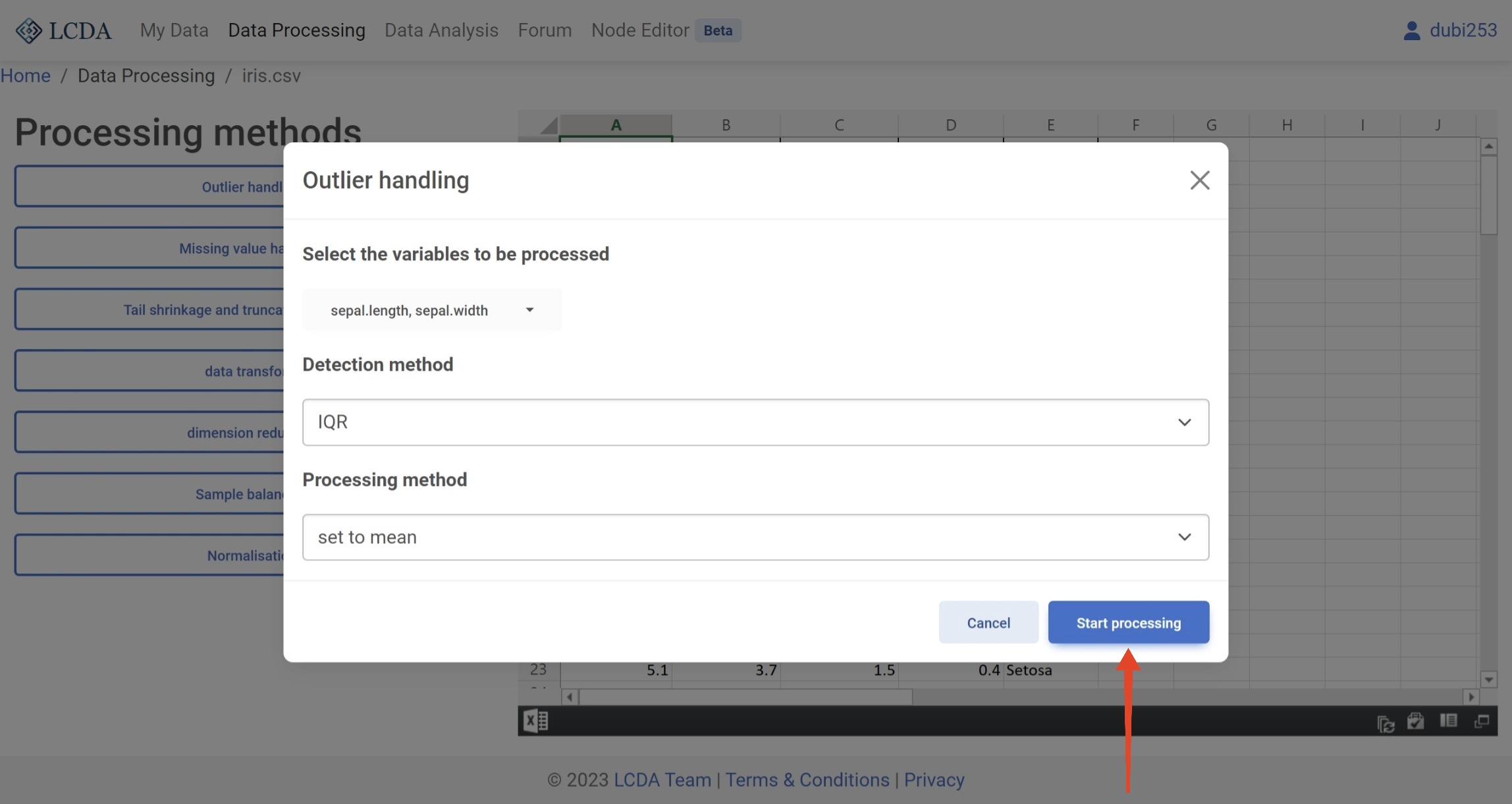
Once the algorithm has completed processing the data, the output will be displayed on the right-hand side of the interface.
At the same time, the processed dataset will be saved and added to your list of datasets. To view or download your new dataset, you can navigate to the
My Datapage.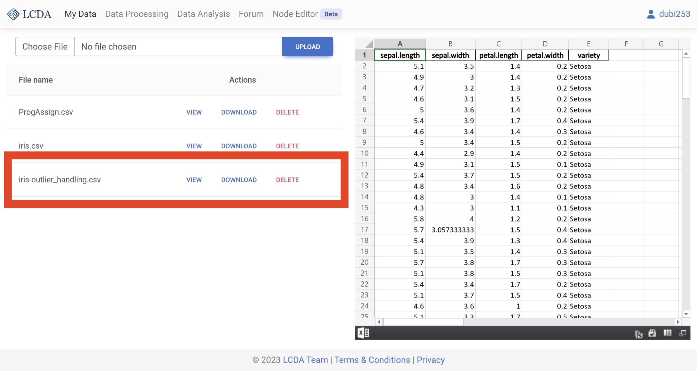
Data Processing Algorithms
Outlier Handling
Description
Outlier handling algorithms are used to identify and handle outliers in a dataset. In statistics, an outlier is a data point that significantly differs from other observations, and may be caused by experimental error or other factors. Outliers can cause serious problems in statistical analysis and can affect the accuracy and reliability of results. Therefore, outlier handling algorithms are essential for identifying and dealing with these problematic data points. These algorithms can help improve the quality of the dataset and ultimately lead to more accurate and reliable analysis results.
Outlier handling algorithms can use various methods for identification and management, including statistical-based, machine learning-based, and deep learning-based approaches. Common statistical-based methods include the 3σ rule, box plot method, etc. Machine learning-based methods include Local Outlier Factor (LOF), Isolation Forest, etc., while deep learning-based methods include Autoencoder, etc.
When dealing with outliers, it is necessary to choose the appropriate algorithm based on the specific scenario. Sometimes, certain outliers may contain useful information, and therefore require careful consideration and management. In general, through appropriate outlier handling algorithms, the quality of the dataset can be improved, and the accuracy of the results can be enhanced.
Parameters
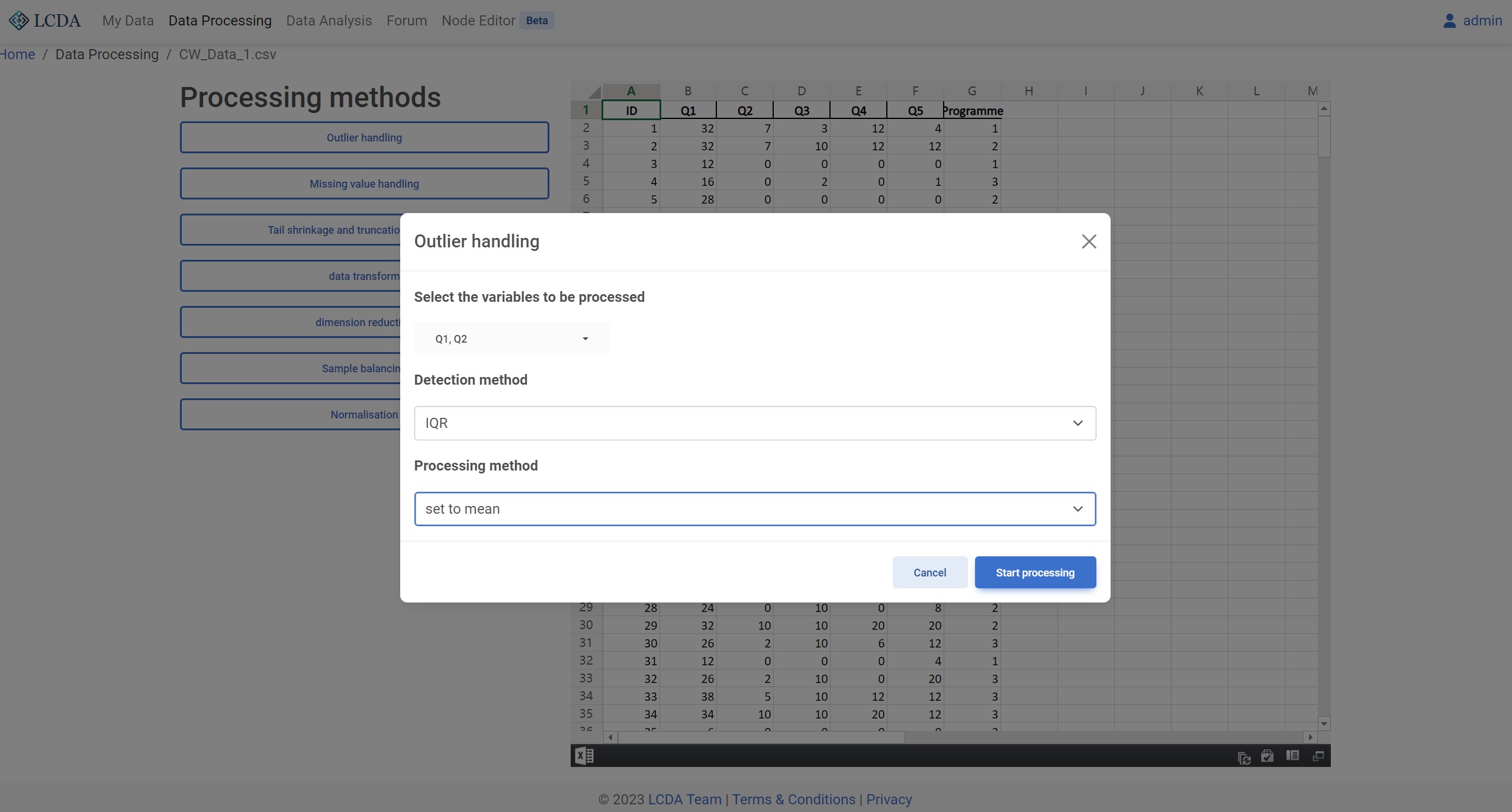
Detection method: Outlier detection method. currently supported 3-sigma, IQR, and MAD three methods.Processing method: Outlier processing method. Currently supportsset to null,set to mean, andset to medianthree methods.
Previews
Missing Value Handling
Description
Missing value processing refers to the process of handling missing values in a dataset. In data analysis and machine learning tasks, missing values are a common problem. The existence of missing values may be due to errors in the data collection process, human omissions, or other factors. If missing values are not handled, they will affect the accuracy and reliability of data analysis and machine learning models.
Methods for missing value processing include deletion, imputation, and prediction. Deletion refers to directly deleting data rows or columns that contain missing values. This method may reduce the amount of data but may make the dataset incomplete and lose useful information. Imputation refers to using existing data to infer missing values. Imputation methods include mean imputation, median imputation, regression imputation, and interpolation. Prediction refers to using machine learning models to predict missing values. This method requires training machine learning models with existing data and then using the models to predict missing values.
When choosing a missing value processing method, factors to consider include the nature of the data, the cause of data missing, and the bias that processing methods may introduce. Through appropriate missing value processing methods, the accuracy and reliability of data analysis and machine learning models can be improved.
Parameters
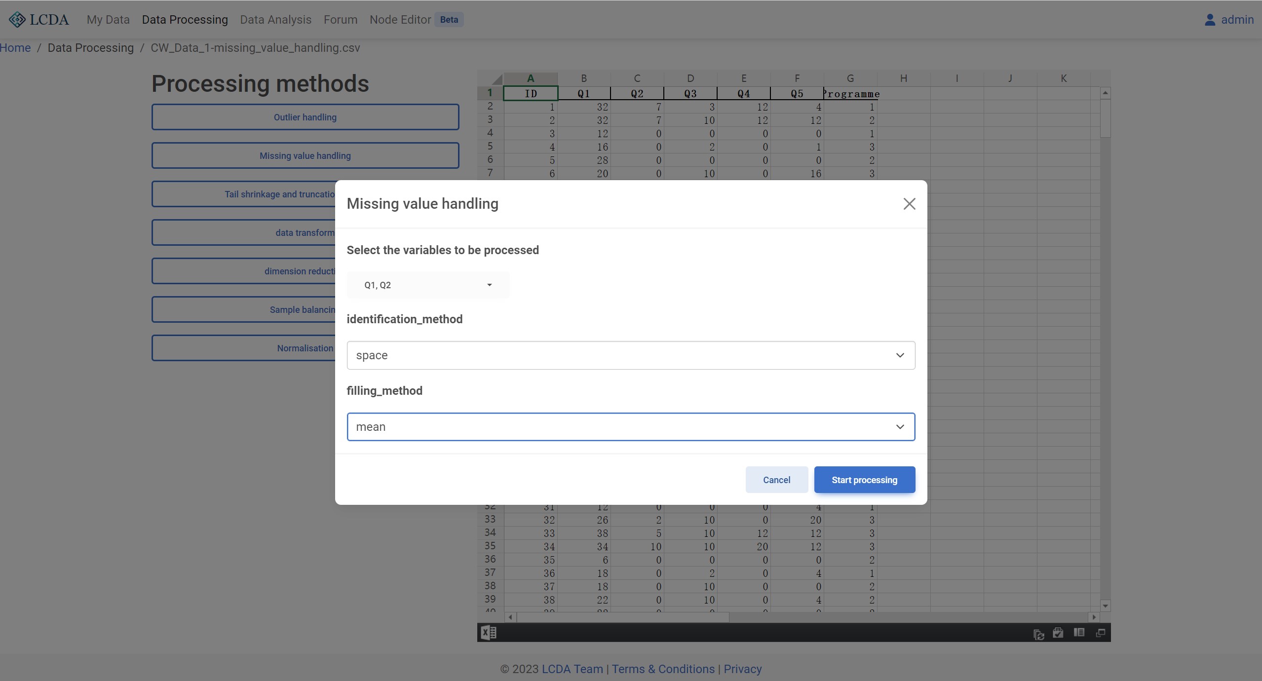
identification method: Missing value detection method. Currently supportsempty,space,NoneandNon-numericfour methods.filling method: missing value processing method. Currently supportsmean,median, andmodethree methods.
Previews
Tail Shrinkage and Truncation Processing
Description
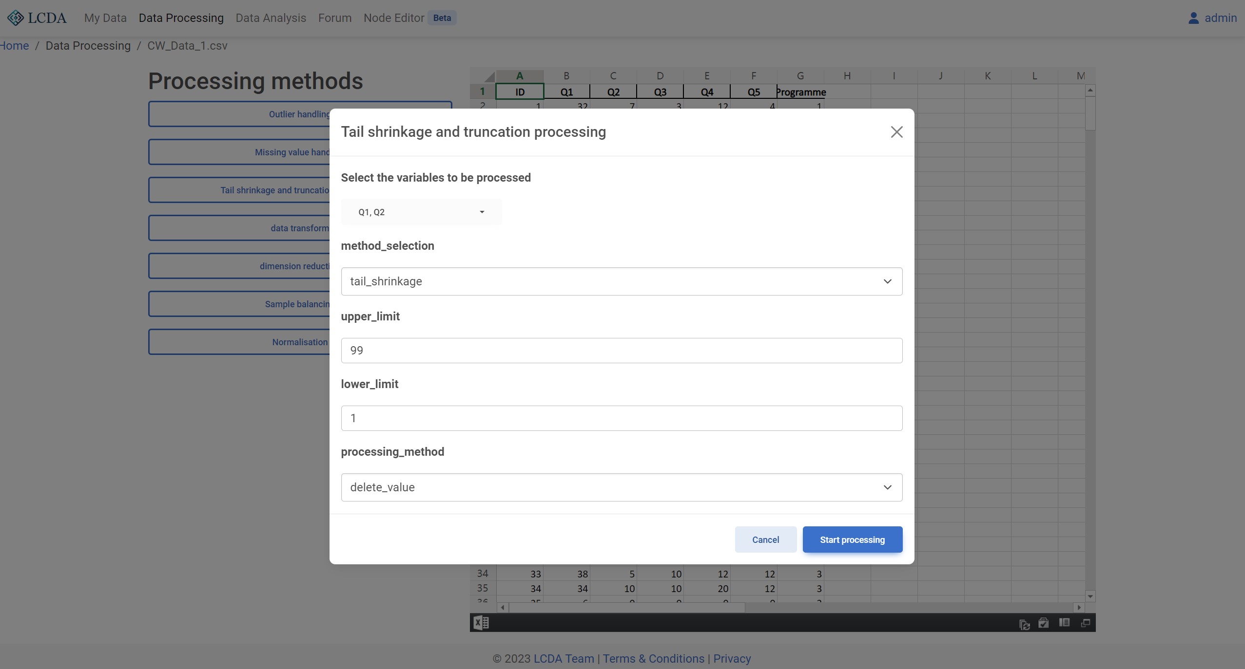
When there is sufficient sample data, it is common to perform shrinkage or truncation on continuous variables to eliminate the influence of extreme values on research. The purpose of shrinkage or truncation is to make the extreme values in the dataset closer to the central value, thereby making the dataset more consistent with the normal distribution. The data values that fall outside of a specific percentile range for the variable are processed after being sorted from smallest to largest. The standard for processing is below the lower limit and beyond the upper limit. Shrinkage replaces these values with their specific percentile values, while truncation directly deletes the values.
Parameters
method_selection: Tail shrinkage and truncation processing method. Currently supportstail_shrinkageandtail_truncationtwo methods.upper_limit: Upper limit of the tail shrinkage and truncation processing. Data types are numeric.lower_limit: Lower limit of the tail shrinkage and truncation processing. Data types are numeric.processing_method: Tail shrinkage and truncation processing method. Currently supportsdelete_valueanddelete_rowtwo methods.
Previews
Data Transformation
Description
Data transformation refers to a process of manipulating or processing the data in the original dataset to extract or modify the information or features contained therein. In the fields of data analysis and machine learning, data transformation is an important step in data preprocessing, which can be used for tasks such as data dimensionality reduction, feature extraction, anomaly detection, and data smoothing.
Parameters
transform_method: Data conversion method. Currently, FFT and IFFT (Inverse Fast Fourier Transform) are supported.
Previews
![]()
Dimension Reduction
Description
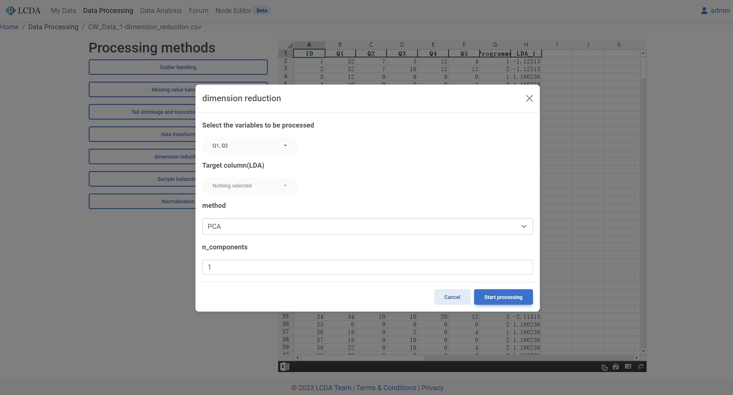
Dimensionality reduction refers to the process of mapping data from a high-dimensional space to a low-dimensional space while preserving the essential features of the original dataset. In the field of data analysis and machine learning, high-dimensional datasets often lead to a significant increase in computational complexity and difficulty in visualizing and interpreting the data. Therefore, dimensionality reduction can effectively reduce the dimensionality of the dataset, improve data processing efficiency and interpretability, and also reduce the risk of overfitting and improve the generalization ability of machine learning models.
Parameters
method: Dimensionality reduction method. Currently supports PCA and LDA two methods.n_components: Number of components to keep. Data types are numeric.
Previews
Sample Balancing
Description
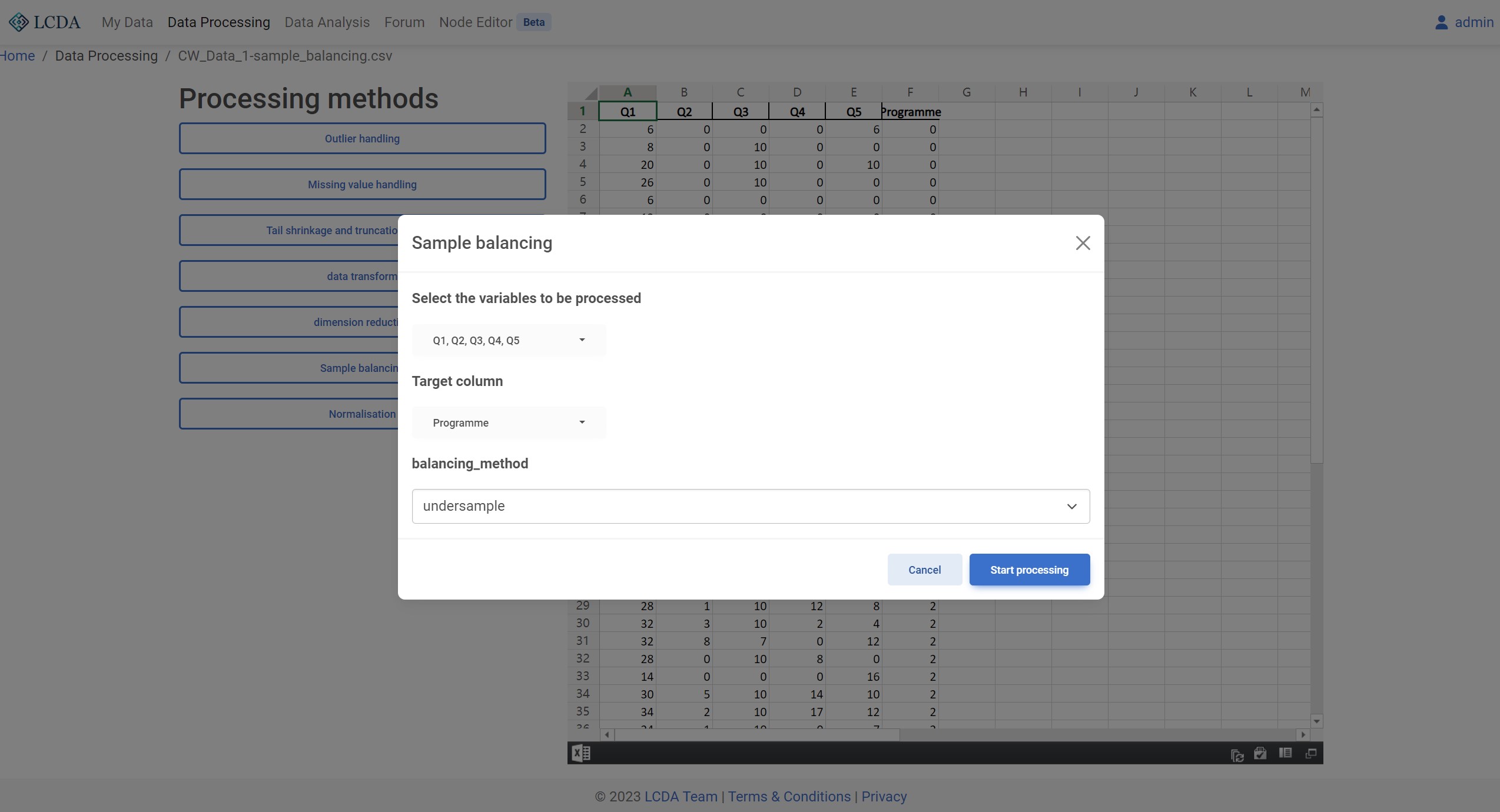
Sample balance refers to the adjustment of sample sizes in each category of a dataset to achieve a more even distribution. In machine learning and data analysis, sample balance is an important preprocessing step because imbalanced datasets can lead to biased results and affect the performance and accuracy of models.
Sample balance can be achieved through various methods, such as undersampling, oversampling, and synthetic sampling. Undersampling involves randomly removing samples from the class with a larger sample size to achieve balance. Oversampling involves duplicating or synthesizing new samples for the class with a smaller sample size. Synthetic sampling involves using generative models such as SMOTEENN to generate new samples to increase sample size and balance different classes.
Sample balance can improve model performance and accuracy while reducing bias due to imbalanced samples. However, excessive sample balance may lead to overfitting, so it is necessary to adjust and balance based on specific situations.
Parameters
balancing_method: Sample balancing method. Currently supportsundersample(RandomUnderSampler),oversample(RandomOverSampler) andcombined(SMOTEENN) three methods.
Previews
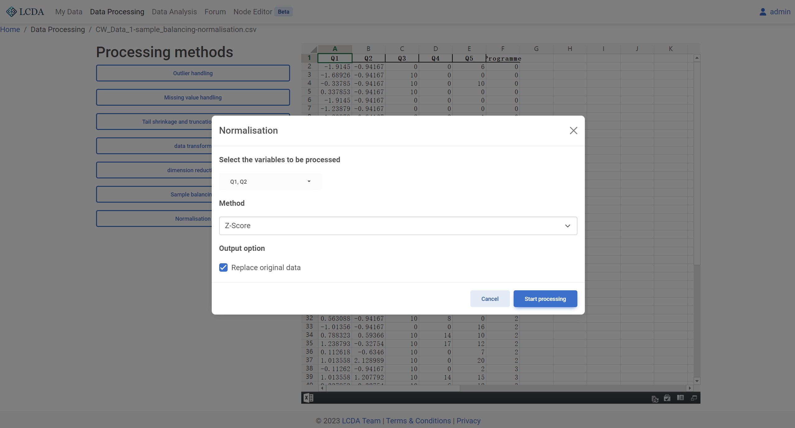
Normalization
Description
Data standardization refers to the process of transforming raw data to conform to a certain standard or specification, making it easier to compare and analyze. The most common method of data standardization is to transform the data into a standard normal distribution with a mean of 0 and a variance of 1, or to scale the data within a certain range.
The main purpose of data standardization is to eliminate differences in units and scales among the data, making comparisons between different variables more fair. For example, if two variables have vastly different ranges of values, the comparison between them may be subject to significant errors. Standardizing the data can eliminate such errors and make the data more reliable and interpretable.
Data standardization is a necessary step in many data analysis and machine learning tasks, such as clustering analysis, regression analysis, and neural networks. Common methods of data standardization include z-score normalization, min-max normalization, and mean-variance normalization.
Parameters
Previews