Data Analysis

Data Analysis helps you to analyze your data on top of Data Processing. Data Analysis provides various algorithms and models used in economics, medicine, social science and Machine Learning, etc.

This chapter will tell you how to analyze data with LCDA, with all the information about the algorithms we provide.

Analysis Steps

1. Click on Data Analysis in the navigation bar above to go to the data analysis page.

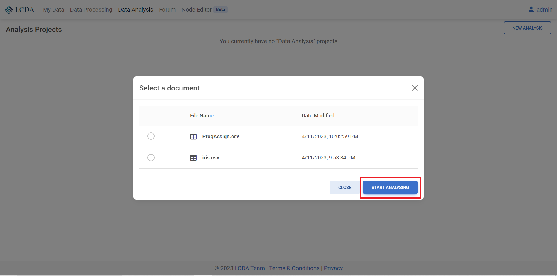
2. Once logged in, click on NEW ANALYSIS in the top right corner, here we select the dataset iris.csv and click on START ANALYSING to start the analysis of the data.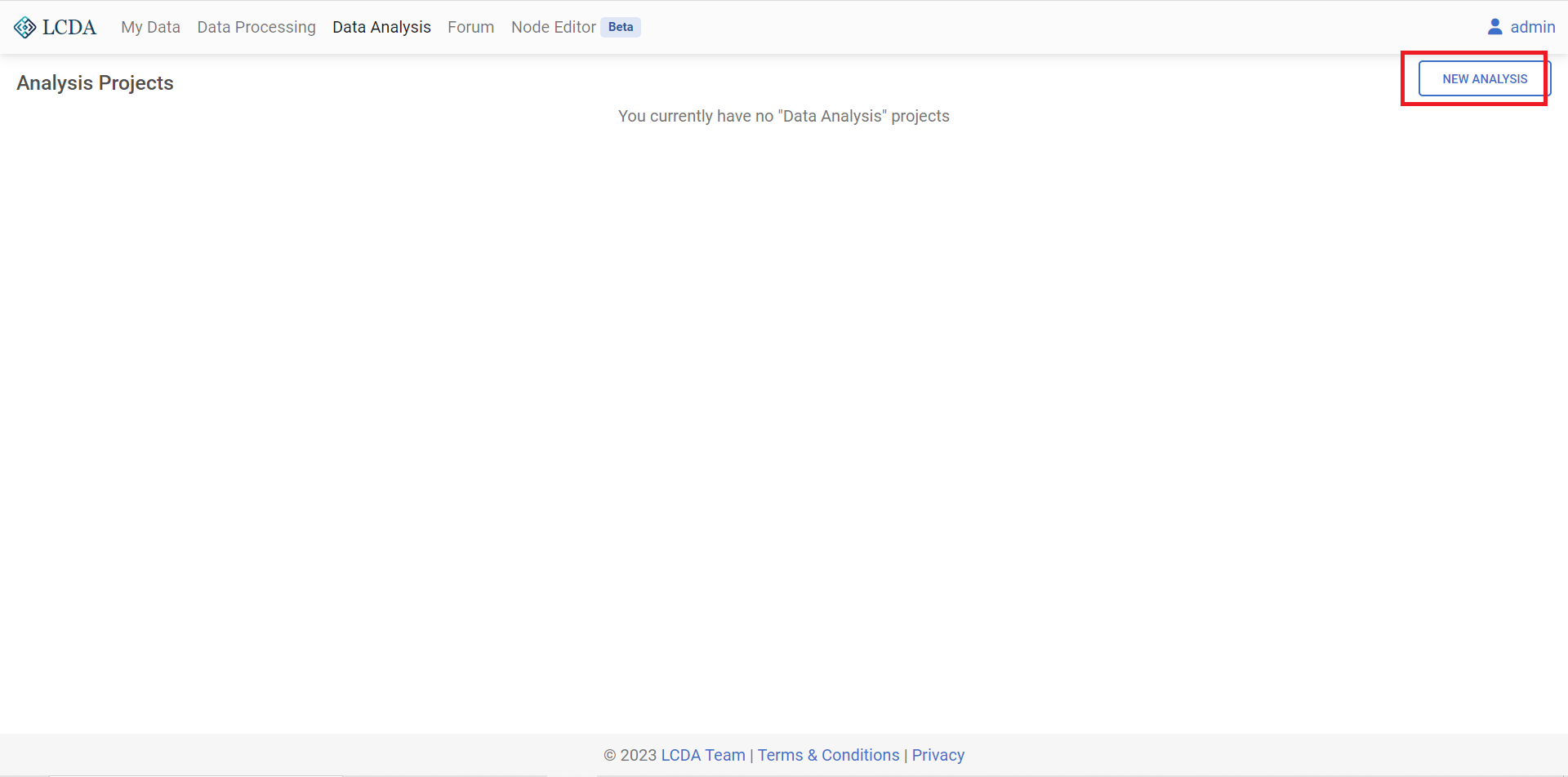

3. The project page firstly displays the project's analysis results Analysis results and the algorithm selection area Choose algorithm.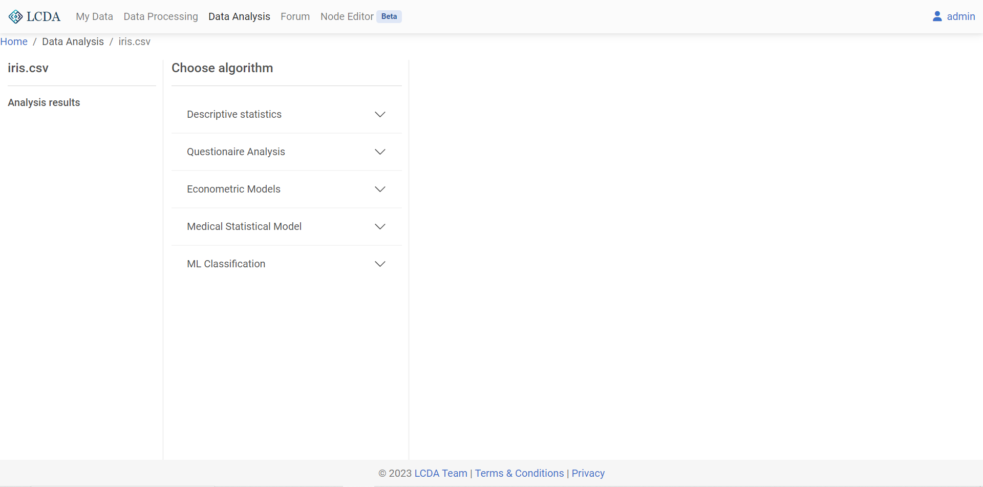

   

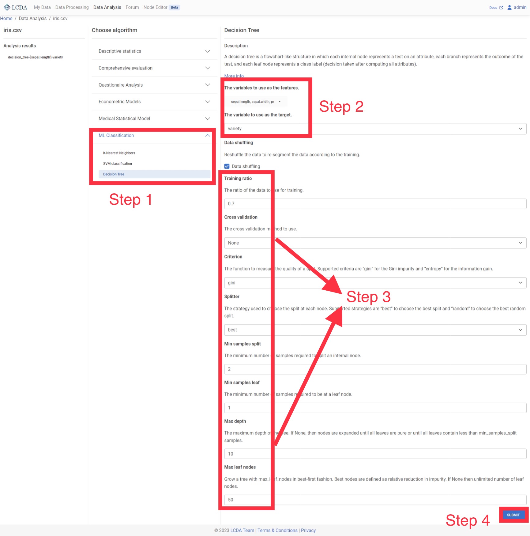
   In the algorithm selection area, the data analysis algorithms and models are classified into several categories. Here we will apply the KNN classification algorithm to the iris dataset, so we click on ML Classification and select K-Nearest Neighbors. A description of the algorithm, the available parameters and the corresponding description will be displayed on the right.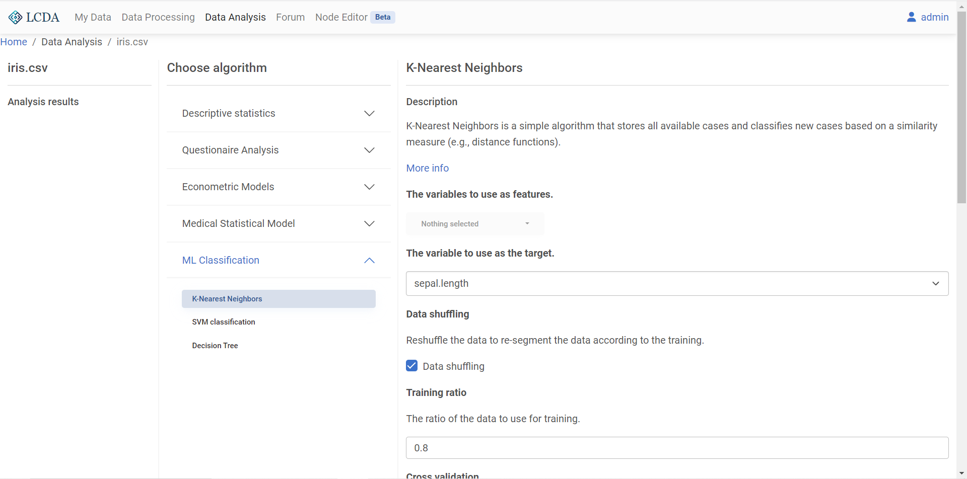 Once you have configured the parameters, click SUBMIT in the bottom right corner at the end of the page to submit the algorithm and parameters.

4. Once you have submitted your algorithm, you can see the analysis report for the algorithm you have just run in the Analysis results on the left hand side. Click on the report to view it on the right.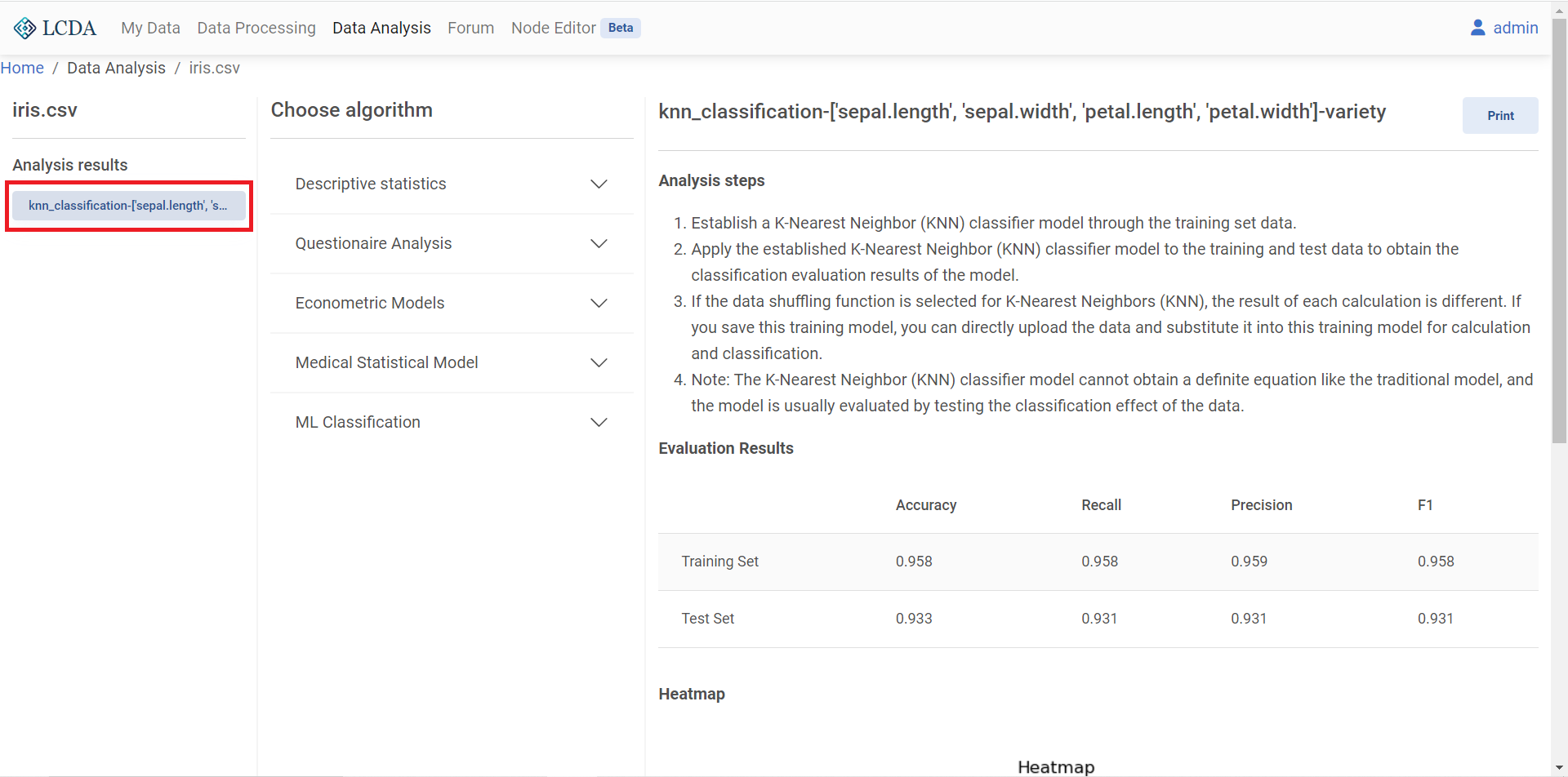

5. The Print button on the top right of the report provides a full screen view and download of the report.

Algorithms

Descriptive Statistics

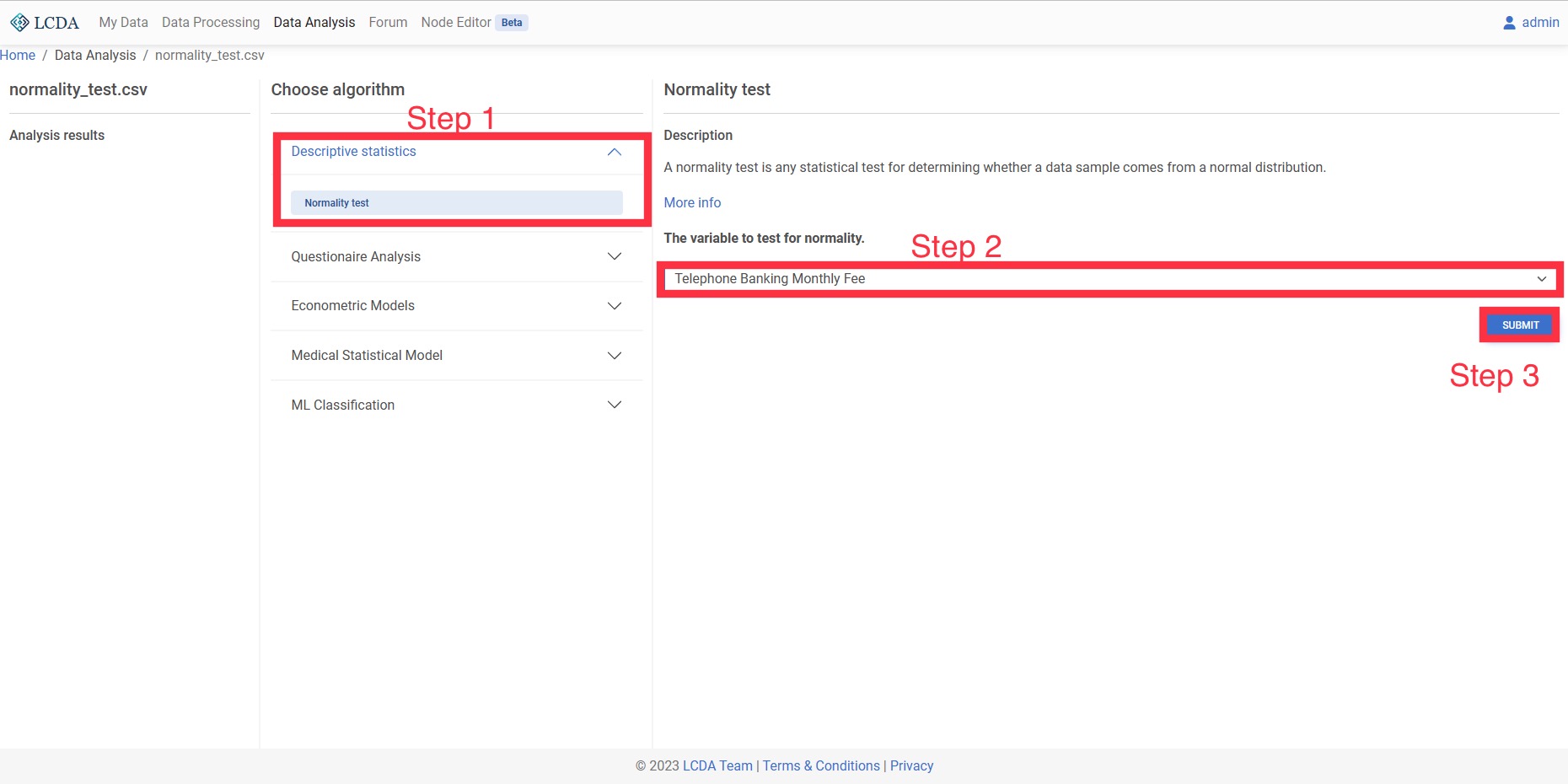
Normality Test

A normality test is any statistical test for determining whether a data sample comes from a normal distribution.

Input and Output

• Input: One or more quantitative variables
• Output: The results of the model test (with data satisfying/not satisfying a normal distribution)

Example Case

Comprehensive Evaluation

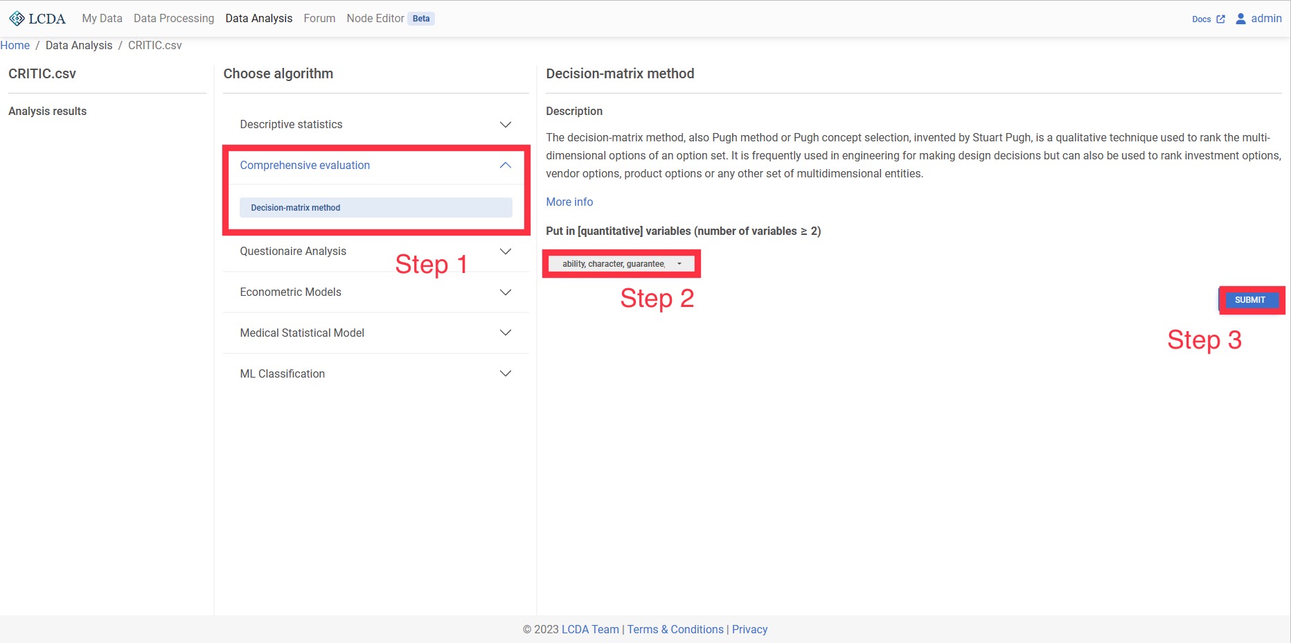
CRITIC weighting method

The CRITIC weighting method is an objective weighting method. The idea is to use two indicators, which are contrast intensity and conflictiveness. Contrast intensity is expressed by standard deviation, if the standard deviation of the data is larger, it means more fluctuation, and the weight will be higher; conflict is expressed by correlation coefficient, if the value of correlation coefficient between indicators is larger, it means less conflict, and then its weight will be lower. For the comprehensive evaluation of multiple indicators and multiple objects, the CRITIC method eliminates the influence of some indicators with strong correlation and reduces the overlap of information between indicators, which is more conducive to obtaining credible evaluation results.

Input and Output

• Input: at least two or more quantitative variables (can be positive or negative, but do not standardize)

• Output: Enter the values of the weights corresponding to the quantitative variables

Example Case

Questionnaire Analysis

Reliability Analysis

Reliability analysis is mainly used to examine the stability and consistency of the results measured by the scale in the questionnaire, that is, to test whether the scale samples in the questionnaire are reliable and credible. The scale question type is the option of the question, which is set according to the level of statement. For example, our love for mobile phones has changed from very fond of to dislike. The most famous scale in the scale is the Likert 5-level scale. The options of this scale are mainly divided into "strongly agree", "agree", "not sure", "disagree", "very disagree" five answers, recorded as 5, 4, 3, 2, 1 respectively.

Input and Output

• Input: At least two or more quantitative variables or ordered fixed categories of variables, generally requiring data to be scale data
• Output: Reliability of the reliability of the collection questionnaire scales

Econometric Models

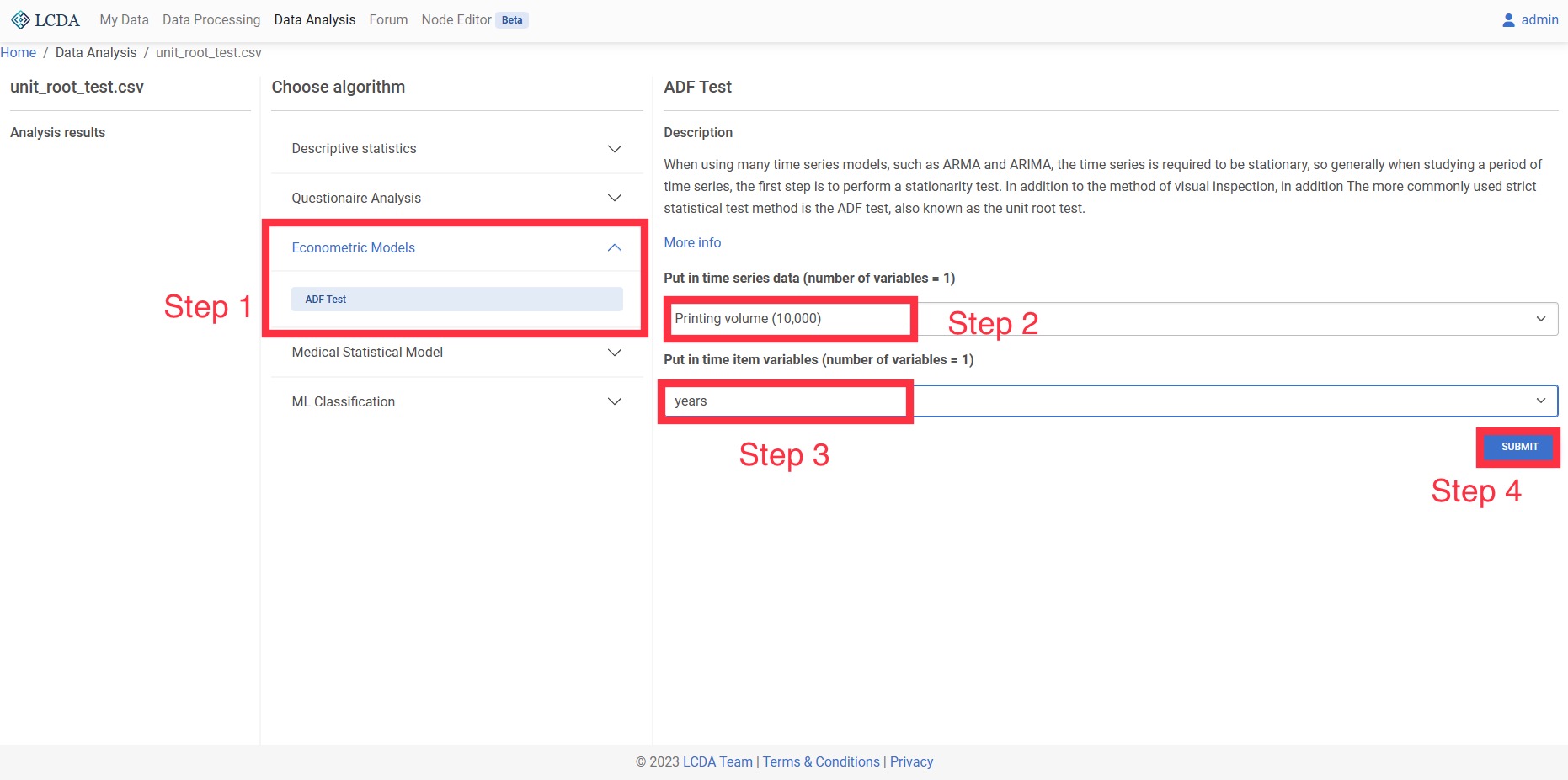
ADF Test

When using many time series models, such as ARMA and ARIMA, the time series is required to be stationary, so generally when studying a period of time series, the first step is to perform a stationarity test. In addition to the method of visual inspection, in addition The more commonly used strict statistical test method is the ADF test, also known as the unit root test.

Input and Output

• Input: 1 quantitative variable for time series data
• Output: Sequence data is smoothed at several orders of differencing

Example Case

Medical Statistical Model

Bland-Altman Method

A method for visual consistency checking. Its principle is an intuitive method to draw graphs using the difference, mean and 95% consistency (LoA) of the results of the two methods, so as to determine whether the results of the two methods are consistent.

Input and Output

• Input: Two quantitative variables representing the two methods
• Output: Bland-Altman graph and whether there is consistency in the approach.

Example Case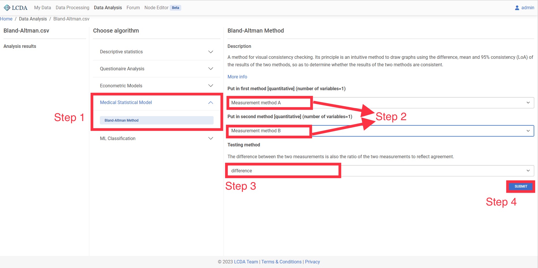

ML Classification

K-Nearest Neighbors

K-Nearest Neighbors is a simple algorithm that stores all available cases and classifies new cases based on a similarity measure (e.g., distance functions).

Input and Output

• Input: The variables as features are fixed or quantitative variables, and the variable as target is a fixed variable.

• Output: The classification results of the model and the evaluation effect of the model classification.

Parameter Options

• Data Shuffling: Whether to shuffle data randomly
• Training Ratio: Ratio of training data to the whole dataset
• Cross Validation: The number of equal sized subsamples randomly partitioned from the original sample. Each subsample will be retained as the validation data for testing the model, and the remaining subsamples will be used as training data
• Number of Neighbors: Number of neighbors to use
• Weights: Weight function used in prediction. Selection values:
  • uniform: Uniform weights. All points in each neighborhood are weighted equally
  • distance: Weight points by the inverse of their distance. in this case, closer neighbors of a query point will have a greater influence than neighbors which are further away
• Algorithm: Algorithm used to compute the nearest neighbors. Selection values:
  • auto: will attempt to decide the most appropriate algorithm based on the values passed
  • ball_tree: will use BallTree
  • kd_tree: will use KDTree
  • brute: will use a brute-force search Note: fitting on sparse input will override the setting of this parameter, using brute force
• Leaf Size: Leaf size passed to BallTree or KDTree. This can affect the speed of the construction and query, as well as the memory required to store the tree. The optimal value depends on the nature of the problem
• P: Power parameter for the Minkowski metric. When p = 1, this is equivalent to using manhattan_distance (l1), and euclidean_distance (l2) for p = 2. For arbitrary p, minkowski_distance (l_p) is used

Example Case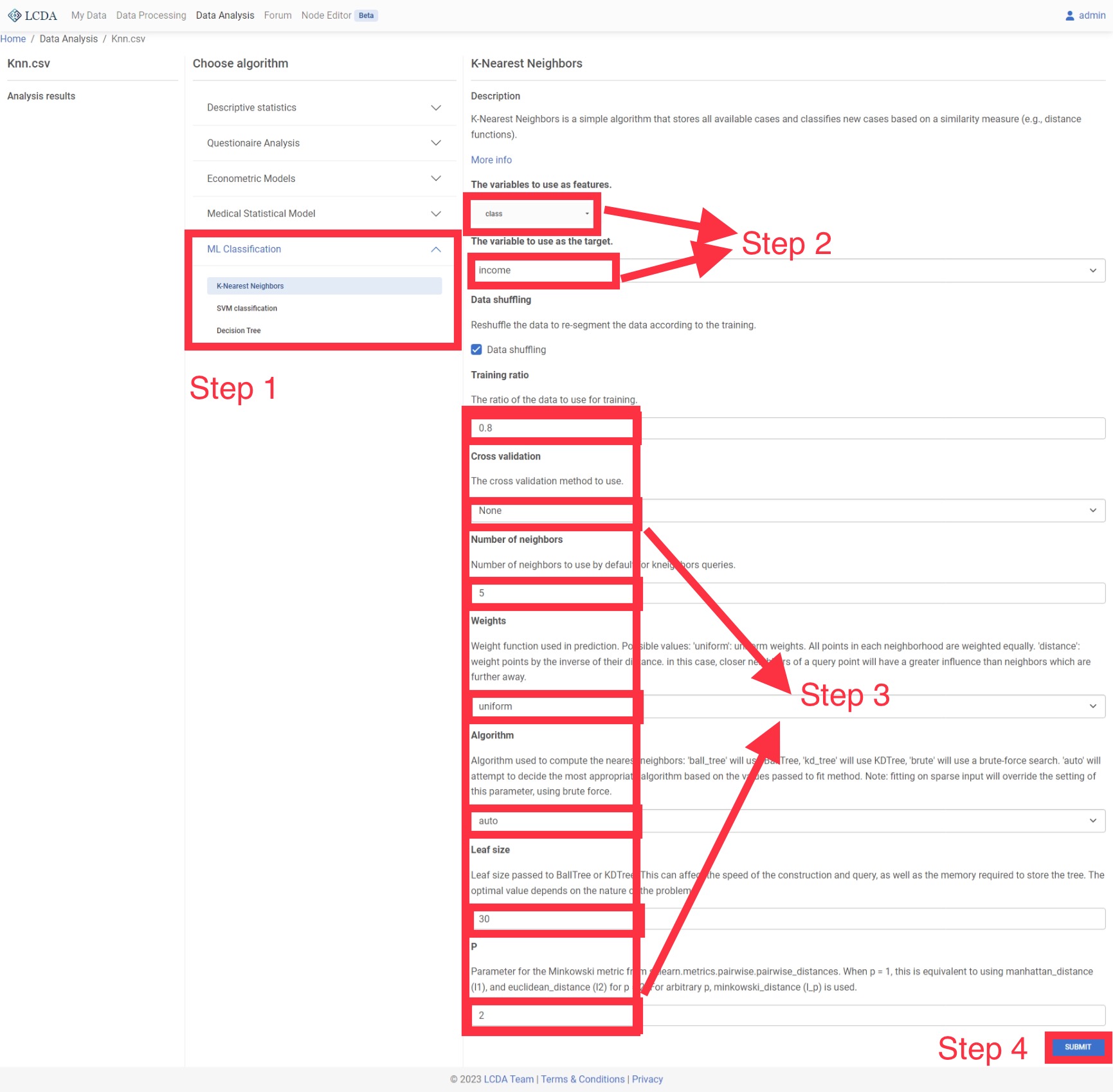

SVM classification

Support vector machine (SVM) is a class of generalised linear classifiers that perform binary classification of data in a supervised learning fashion, with a decision boundary that is a maximum margin hyperplane solved for the learned samples.

Input and Output

• Input: The variables as features are fixed or quantitative variables, and the variable as target is a fixed variable.
• Output: The classification results of the model and the evaluation effect of the model classification.

Parameter Options

• Data Shuffling: Whether to shuffle data randomly
• Training Ratio: Ratio of training data to the whole dataset
• Cross Validation: The number of equal sized subsamples randomly partitioned from the original sample. Each subsample will be retained as the validation data for testing the model, and the remaining subsamples will be used as training data
• Penalty Coefficient: Regularization parameter. The strength of the regularization is inversely proportional to C. Must be strictly positive. The penalty is a squared l2 penalty
• Kernel Algorithm: Specifies the kernel type to be used in the algorithm
• Error Convergence Conditions: Tolerance for stopping criterion
• Maximum Number of Iterations: Hard limit on iterations within solver, or -1 for no limit

Example Case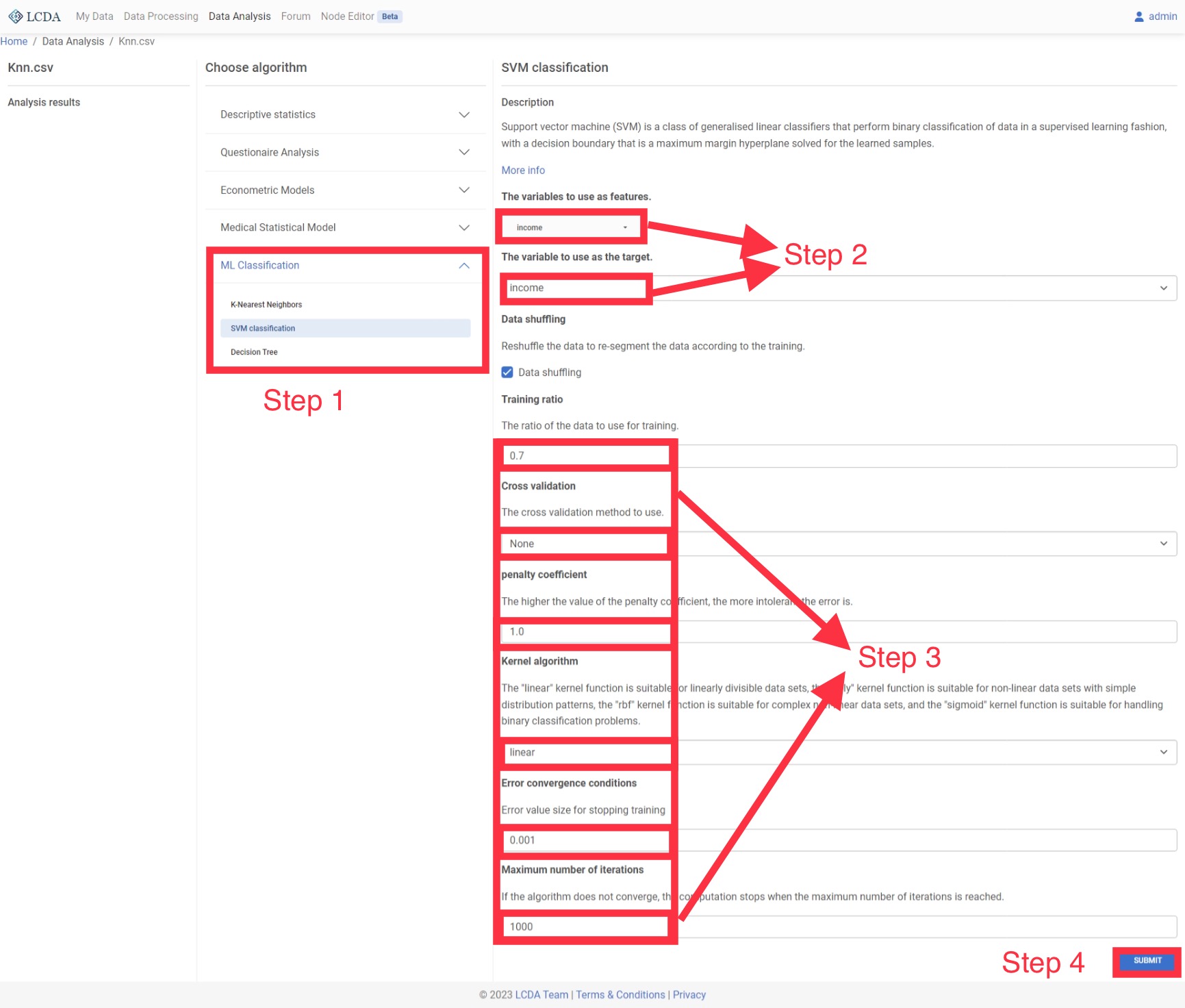

Decision Tree

A decision tree is a flowchart-like structure in which each internal node represents a test on an attribute, each branch represents the outcome of the test, and each leaf node represents a class label (decision taken after computing all attributes).

Input and Output

• Input: The variables as features are fixed or quantitative variables, and the variable as target is a fixed variable.
• Output: The classification results of the model and the evaluation effect of the model classification.

Parameter Options

• Data Shuffling: Whether to shuffle data randomly
• Training Ratio: Ratio of training data to the whole dataset
• Cross Validation: The number of equal sized subsamples randomly partitioned from the original sample. Each subsample will be retained as the validation data for testing the model, and the remaining subsamples will be used as training data
• Criterion: The function to measure the quality of a split. Supported criteria are:
  • gini: for the Gini impurity
  • entropy: for the Shannon information gain
• Splitter: The strategy used to choose the split at each node. Supported strategies:
  • best: choose the best split
  • random: choose the best random split
• Min Samples Split: The minimum number of samples required to split an internal node:
  • If int, then consider Min Samples Split as the minimum number.
  • If float, then Min Samples Split is a fraction and ceil(Min Samples Split * n_samples) are the minimum number of samples for each split.
• Min Samples Leaf: The minimum number of samples required to be at a leaf node. A split point at any depth will only be considered if it leaves at least Min Samples Leaf training samples in each of the left and right branches. This may have the effect of smoothing the model, especially in regression.
  • If int, then consider Min Samples Leaf as the minimum number.
  • If float, then Min Samples Leaf is a fraction and ceil(Min Samples Leaf* n_samples) are the minimum number of samples for each node. .. versionchanged:: 0.18 Added float values for fractions.
• Max Depth: The maximum depth of the tree. If None, then nodes are expanded until all leaves are pure or until all leaves contain less than Min Samples Split samples.
• Max leaf nodes: Grow a tree with Max leaf nodes in best-first fashion. Best nodes are defined as relative reduction in impurity. If None then unlimited number of leaf nodes.

Example Case